How to use Charlie Sheen to improve your estimating…
Monte Carlo simulations are cool – very cool. in this post I am going to try and out-do Kailash Awati in trying to explain what they are. You see, I am one of these people who’s eyes glaze over the minute you show me any form of algebra. Kailash recent wrote a post to explain Monte Carlo to the masses, but he went and used a mathematical formula (he couldn’t help himself), and thereby lost me totally. Mind you, he used the example of a drunk person playing darts. This I did like a lot and gave me the inspiration for this post.
So here is my attempt to explain what Monte Carlo is all about and why it is so useful.
I have previously stated, that vaguely right is better than precisely wrong. If someone asks me to make an estimate on something, I offer them a ranged estimate, based on my level of certainty. Thus for example, if you asked me to guess how many beers per day Charlie Sheen has been knocking back lately, I might offer you an estimate of somewhere between 20 and 50 pints. I am not sure of the exact number (and besides, it would vary on a daily basis anyway) , so I would rather give you a range that I feel relatively confident with, than a single answer that is likely to be completely off base.
Similarly, if you asked me how much a SharePoint project to “improve collaboration” would cost, I would do a similar thing. The difference between SharePoint success and Charlie Sheen’s ability to keep a TV show afloat is that with SharePoint, there are more variables to consider. For example, I would have to make ranged estimates for the cost of:
- Hardware and licensing
- Solution envisioning and business analysis
- Application development
- Implementation
- Training and user engagement
Now here is the problem. A CFO or similar cheque signer wants certainty. Thus, if you give them a list of ranged estimates, they are not going to be overly happy about it. For a start, any return on investment analysis is by definition, going to have to pick a single value from each of your estimates to “run the numbers”. Therefore if we used the lower estimate (and therefore lower cost) for each variable, we would inevitably get a great return on investment. If we used the upper limit to each range, we are going to get a much costlier project.
So how to we reconcile this level of uncertainty?
Easy! Simply run the numbers lots and lots (and lots) of times – say, 100,000 times, picking random values from each variable that goes into the estimate. Count the number of times that your simulation is a positive ROI compared to a negative one. Blammo – that’s Monte Carlo in a nutshell. It is worth noting that in my example, we are assuming that all values between the upper and lower limits are equally likely. Technically this is called a uniform distribution – but we will get to the distribution thing in a minute.
As a very crappy, yet simple example, imagine that if SharePoint costs over $250,000 it will be considered a failure. Below are our ranged estimates for the main cost areas:
| Item | Lower Cost | Upper Cost |
| Hardware and licensing | $50,000 | $60,000 |
| Solution envisioning and business analysis | $20,000 | $70,000 |
| Application development | $35,000 | $150,000 |
| Implementation | $25,000 | $55,000 |
| Training and User engagement | $10,000 | $100,000 |
| Total | $140,000 | $435,000 |
If you add up my lower estimates we get a total of $140,000 – well within our $250,000 limit. However if my upper estimates turn out to be true we blow out to $435,000 – ouch!
So why don’t we pick a random value from each item, add them up, and then repeat the exercise 100,000 times. Below I have shown 5 of 100,000 simulations.
| Item | Simulation 1 | Simulation 2 | Simulation 3 | Simulation 4 | [snip] | Simulation 100,000 |
| Hardware and licensing | 57663 | 52024 | 53441 | 58432 | … | 51252 |
| Solution envisioning and business analysis | 21056 | 68345 | 42642 | 37456 | … | 64224 |
| Application development | 79375 | 134204 | 43566 | 142998 | … | 103255 |
| Implementation | 47000 | 25898 | 25345 | 51007 | … | 35726 |
| Training and User engagement | 46543 | 73554 | 27482 | 87875 | … | 13000 |
| Total Cost | 251637 | 354025 | 192476 | 377768 | … | 267457 |
So according to this basic simulation, only 2 out of 5 shown are below $250,000 and therefore a success according to my ROI criteria. Therefore we were successful only only 40% of the time (2/5 = .4). By that measure, this is a risky project (and we haven’t taken into account discounting for risk either).
“Thats it?”, I hear you say? Essentially yes. All we are doing is running the numbers over and over again and then looking at the patterns that emerge from this. But that is not the key bit to understand. Instead, the most important thing to understand with Monte Carlo properly is to understand probability distributions. This is the bit that people mess up on and the bit that people are far too quick to jump into mathematical formulae.
But random is not necessarily random
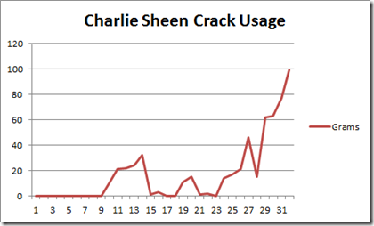
Let’s use Charlie Sheen again to understand probability distributions. If we were to consider the amount of crack he smokes on a daily basis, we could conclude it is between 0 grams and 120 grams. The 120g upper limit is based on what Charlie Sheen could realistically tolerate (which is probably three times the amount of normal humans). If we plotted this over time, it might look like the example below (which is the last 31 days):
So to make a best guess at the amount he smokes tomorrow, should we pick random values between 0 and 120 grams? I would say not. Based on observing the chart above, you would be likely to choose values from the upper end of the range scale (lately he has really been hitting things hard and we all know what happens when he hangs with starlets from the adult entertainment industry).
That’s the trick to understanding a probability distribution. If we simply chose a random value it would likely not be representative of the recent range of values. We still have to pick a value from a range of possibilities, but some values are more likely than others. We are not truly picking random values at all.
The most common probability distribution people use is the old bell curve – you probably saw it in high school. For many variables that go into a monte carlo, it is a perfectly fine distribution. For example, the average height of a human male may be 5 foot 6. Some people will be larger and some will be smaller, but you would find that there would be more people closer to this mid-point than far away from it, hence the bell shape.

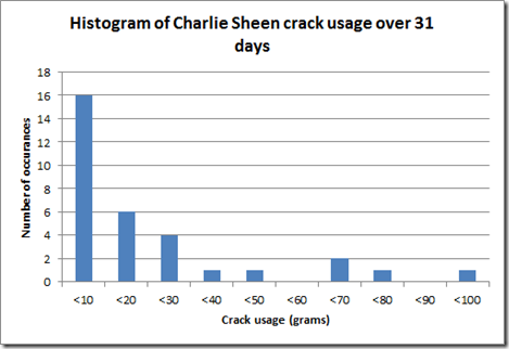
Let’s see what Charlie Sheen’s distribution looks like. Since we have our range of values, for each days amount of crack usage, let’s divide up crack usage into ranges of grams and see how much Charlie has consumed. The figure is below:
| Amount | Daily occurrences | % |
| 0-10g | 16 | 50% |
| 10-20g | 6 | 19% |
| 20-30g | 4 | 13% |
| 30-40g | 1 | 3% |
| 40-50g | 1 | 3% |
| 50-60g | 0 | 0% |
| 60-70g | 2 | 6% |
| 70-80g | 1 | 3% |
| 80-90g | 0 | 0% |
| 90-100g | 1 | 3% |
| 100-120g | 0 | 0% |
As you can see, according to the 50% of the time Charlie was not hitting the white stuff particularly hard. There 16 occurrences where Charlie ingested less than 10 grams. What sort of curve does this make? The picture below illustrates it.
Interesting huh? If we chose random numbers according to this probability distribution, chances are that 50% of the time, we would get a value between 0 and 10 grams of crack being smoked or shovelled up his nasal passages. Yet when we look at the trend of the last 10 days, one could reasonably expect that its likely that tomorrows value would be significantly higher than zero. In fact there were no occurrences at all of less than 10 grams in a single day in the last 10 days.
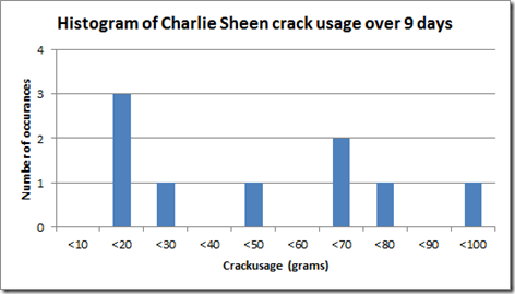
Now let’s change the date range, and instead look at Charlie’s last 9 days of crack usage. This time the distribution looks a bit more realistic based on recent trends. Since he has not been well behaved lately, there were no days at all where his crack usage was less than 10 grams. In fact 4 of the 9 occurrences were over 60 grams.
| Amount | Daily occurrences | % |
| 0-10g | 0 | 0% |
| 10-20g | 3 | 33% |
| 20-30g | 1 | 11% |
| 30-40g | 0 | 0% |
| 40-50g | 1 | 11% |
| 50-60g | 0 | 0% |
| 60-70g | 2 | 22% |
| 70-80g | 1 | 11% |
| 80-90g | 0 | 0% |
| 90-100g | 1 | 11% |
| 100-120g | 0 | 0% |
This time, utilising a different set of reference points (9 days instead of 31), we get very different “randomness”. This gets to one of the big problems with probability distributions which Kailash tells me is called the Reference class problem. How can you pick a representative sample? In some situations completely random might actually be much better than a poorly chosen distribution.
Back to SharePoint…
So imagine that you have been asked to estimate SharePoint costs and you only have vague, ranged estimates. Lets also assume that for each of the variables that need to be assigned an estimate, you have some idea of their distribution. For example if you decide that SharePoint hardware and licensing really could be utterly random between $50000-$60000 then pick a truly random value (a uniform distribution) from the range with each iteration of the simulation. But if you decide that its much more likely to come in at $55000 than it is $50000, then your “random” choice will be closer to the middle of the range more often than not – a normal distribution.
So the moral of the story? Think about the sort of distribution that each variable uses. It’s not always a bell curve. its also not completely random either. In fact you should strive for a distribution that is the closest representation of reality. Kailash tells me that a distribution “should be determined empirically – from real data – not fitted to some mathematically convenient fiction (such as the Normal or Unform distributions). Further, one should be absolutely certain that the data is representative of the situation that is being estimated.”
Since SharePoint often relies on some estimations that offer significant uncertainty, a Monte Carlo simulation is a good way to run the numbers – especially if you want to see how many variables with different probability distributions combine to produce a result. Run the simulation enough times, you will produce a new probability distribution that represents all of these variables.
Just remember though – Charlie Sheen reliably demonstrates that things are not often predictable and that past values are no reliable indicator of future values. Thus a simulation is only as good as your probability distributions in the first place
Thanks for reading
Paul Culmsee
p.s A huge thanks to Kailash for checking this post, offering some suggestions and making sure I didn’t make an arse of myself.


March 14th, 2011 at 6:28 pm |
Brilliant stuff mate. Very well done!
March 15th, 2011 at 8:59 pm |
[…] the Blogosphere How to Use Charlie Sheen to Improve Your Estimating… (Clever Workarounds) Monte Carlo simulations are cool – very cool. in this post I am going to try […]
March 15th, 2011 at 9:02 pm |
[…] the BlogosphereHow to Use Charlie Sheen to Improve Your Estimating… (Clever Workarounds)Monte Carlo simulations are cool – very cool. in this post I am going to […]
March 17th, 2011 at 2:07 am |
Nice; but how do you get the historical data in the first place?
I’ve been trying to figure out how we can capture estimates and actual times for development projects – but usually the project changes between estimate and execution so much that it’s very difficult to get good correlation.
March 17th, 2011 at 5:48 pm |
Great question and thats at the heart of the problem. The scrum world alleviates this somewhat by the fixed nature of a sprint, which would make such backtesting easier. But a wicked or learning problem by definition does not necessarily lend itself to this.
But at the end of the day you are only as good as your distribution. Calibrating estimates can help for some aspects of bias and assuming you have done that, time estimates may well follow a normal(ish) type of distrbution.
I wanted to modify my ROI spreadsheet to allow you to select a distribution and use ranged estimates, but it got a little too hard :-\
regards
Paul
March 17th, 2011 at 10:33 pm |
So, where’s the downloadable Excel sheet that we can plug our numbers and distributions into? 😉
January 22nd, 2012 at 8:27 am |
[…] cartoon was from Paul Culmsee and supports his blog series on estimating and this one on Charlie Sheen (trust me you will […]
August 5th, 2012 at 10:44 pm |
[…] “Why is that system so slow?” Another brilliantly entertaining and educational piece is this one on Monte Carlo simulation. (Full Disclosure: Paul is a good friend of mine and we’ve co-written […]